StarTrailCUDA: GPU-Accelerated Rendering of Night-Sky Star Trails Video - Milestone Report
Team Members: Zijun Yang <[email protected]> and Jiache Zhang <[email protected]>
Project Home Page: https://blog.zjyang.dev/StarTrailCUDA/

LIST OF WORK COMPLETED SO FAR
We explored different star trail algorithms:
MAX: The MAX algorithm maintains an accumulated per-pixel maximum with a small decay so that bright pixels persist as trails. (Jiache Zhang)
AVERAGE: The AVERAGE algorithm sums frames within a sliding window and outputs the per-pixel average, equally combining recent frames. (Jiache Zhang)
EXPONENTIAL: The EXPONENTIAL algorithm maintains an exponential moving average of frames (
LINEAR: The LINEAR algorithm keeps a fixed-size deque of recent frames and applies linearly decreasing weights with element-wise maxima across weighted frames. The cost of LINEAR algorithm is
LINEARAPPROX: Uses mathematical heuristics to approximate the LINEAR algorithm with
We explored different implementations:
Baseline: The baseline implementation is a CPU-based, serial decode–render–encode pipeline built with OpenCV that serves as our correctness reference and performance benchmark; it exposes decoding/encoding and per-frame rendering as the primary bottlenecks on high-resolution inputs. (Jiache Zhang)
Baseline with hardware codec: Similar to baseline, but with both video decoding and encoding replaced with hardware-accelerated implementations (using NVENC for encoding and CUVID for decoding) for improved performance. (Jiache Zhang and Zijun Yang)
CUDA: Similar to baseline with hardware codec, but with the rendering phase replaced with pixel-wise parallelism using CUDA kernels for high-performance computation of star trail effects. (Zijun Yang)
PRELIMINARY RESULTS
NOTICE: Most videos on this page are in 4K. If you notice any aliasing, viewing it in full screen usually helps.
Unless otherwise stated, the results are from an AWS EC2 g4dn.xlarge instance (4 vCPUs, 16GB RAM, NVIDIA T4, gp2 storage with 100 IOPS) running LINEARAPPROX algorithm with default parameters.
RENDERING ALGORITHMS
Source Material Selection
Our source material is a high-quality all-night sky recording (non-time-lapse) from YouTube (video source: <https://www.youtube.com/watch?v=Bbp1-p2FoXU>). This video provides excellent clarity and resolution (3840×2160), making it ideal for rendering star trail videos.
We considered alternative sources, particularly examining the database at <https://data.phys.ucalgary.ca/>, which contains comprehensive continuous nighttime recordings from observatories worldwide over recent years. While this database offers extensive and complete data, it presents a significant limitation: the cameras are primarily scientific instruments designed for research purposes rather than high-quality cinematography, resulting in insufficient clarity for star trail rendering. Therefore, we opted for clear videos recorded by amateur astronomy enthusiasts.
Video vs. Image Format Consideration
Theoretically, using video files versus collections of individual images as source media would yield equivalent results. However, storing media in image format requires prohibitively large storage space. Our test video, when stored as an MP4 file, occupies 101.77MB. When each frame of this video is saved in PNG format, the total storage requirement reaches 18GB; even with JPEG compression, it still requires 3.6GB. This storage demand is unacceptable for development and testing environments with limited storage capacity (for example, GHC servers impose a 2GB storage limit per user, insufficient for image-format media storage). Mounting remote storage would introduce additional I/O overhead.
Consequently, we decided to store and process source media in video format to minimize local storage requirements. Additionally, MP4-compressed video maintains sufficient quality without affecting final rendering results, eliminating the need for uncompressed video or image inputs.
MAX Algorithm
The MAX algorithm creates star trails by maintaining a cumulative maximum frame that preserves the brightest pixel values encountered over time. At each frame, the algorithm performs an element-wise maximum operation between the current input frame and the accumulated maximum frame, ensuring that bright stars leave persistent trails while darker background regions remain unaffected.
Key implementation details:
Decay Factor: A decay factor of 0.999 is applied to the accumulated frame before comparison, causing older trails to gradually fade and preventing infinite accumulation of brightness values
Pixel-wise Maximum: For each pixel position, the algorithm selects the maximum value between the decayed accumulated frame and the current frame:
maxFrame = max(maxFrame × 0.999, currentFrame)
While this approach is conceptually simple and straightforward to implement, the practical results are suboptimal. The decay factor of 0.999 is insufficient to prevent excessive accumulation of brightness values over time. As the video progresses, bright points fade too slowly, causing an increasing number of luminous artifacts to persist in the frame. This leads to severe overexposure and blurring effects, where the accumulated trails become overly bright and lose definition. The resulting star trail video appears washed out with poor contrast and indistinct trail boundaries, making it difficult to discern individual star trajectories. Although the MAX algorithm successfully demonstrates the basic concept of trail preservation, its aggressive retention of bright pixels without adequate decay control produces unsatisfactory visual quality.
LINEAR Algorithm
The LINEAR algorithm produces the highest quality star trail effects among all tested approaches by implementing a sophisticated sliding window technique with linear weight decay. This method maintains a fixed-size window of recent frames and applies linearly decreasing weights to create natural-looking trail fade effects.
Key implementation details:
Sliding Window: Maintains a deque of the most recent W frames (where W is the window size), automatically removing the oldest frame when the window is full
Linear Weight Decay: Applies weights ranging from 1.0 (most recent frame) to 1/W (oldest frame in window), creating a smooth linear fade:
weight = (W - i) / WPixel-wise Maximum: For each frame position, performs element-wise maximum operation between the weighted frame and the accumulated result:
accFrame = max(accFrame, weightedFrame)
This approach produces visually superior results with well-defined star trajectories, appropriate trail lengths, and natural fade characteristics. The linear weighting ensures that recent star positions are prominent while older positions gradually diminish, creating realistic motion blur effects that closely resemble long-exposure photography techniques.
However, the algorithm's computational complexity is significantly higher due to the need to maintain and process the entire sliding window for each output frame. In our serial implementation, the LINEAR algorithm requires approximately 1125 seconds to complete rendering, making it impractical for real-time or near-real-time applications. The performance bottleneck stems from the intensive memory operations and repeated maximum computations across the sliding window, highlighting the critical need for parallel optimization techniques.
LINEARAPPROX Algorithm
In the LINEAR algorithm, it is very expensive both in memory and computation to trace back
To solve this issue, we leverage the fact that the exponential function has a derivative of 1 near
, where
Here's a comparison between the ground truth (the blue line) and our heuristic (the green line) under
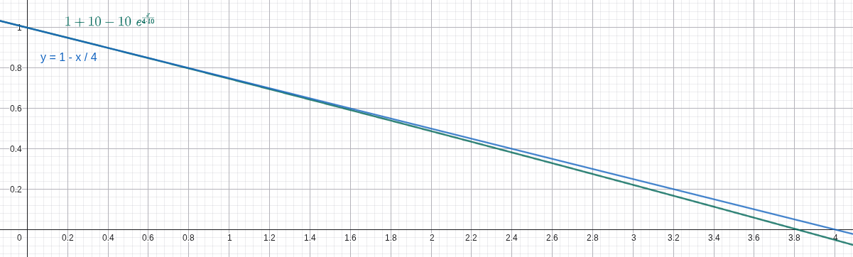
With this heuristic, the new output frame can be approximated using only the last output frame and the new input frame using this formula in
The LINEARAPPROX algorithm looks very similar to the LINEAR algorithm in controlling the tail length and window size except for being slightly darker. We suspect the difference mainly comes from floating point precision and rounding errors. Also, both of us think it actually looks better than the LINEAR algorithm because it emphasizes bright stars and suppresses the darker ones, creating a cleaner video.
In the baseline implementation, we compared the performance difference for the LINEAR algorithm and the LINEARAPPROX algorithm under default parameters given the test input (
BASELINE RENDERER
The baseline implementation serves as our reference CPU-based serial processing pipeline, built entirely around the OpenCV library for comprehensive video processing operations. This implementation provides a clean, modular architecture that handles video input, frame-by-frame rendering computations, and video output encoding in a sequential manner.

Architecture Overview:
Frame Reader Module: Implements a
FrameReaderclass hierarchy that abstracts video input sources, supporting both video files and image folder sequences. The module handles frame extraction, format conversion, and provides a unified interface for accessing sequential video frames regardless of the input format.Video Renderer: Contains the core rendering logic with support for multiple star trail algorithms (MAX, LINEAR, LINEARAPPROX, etc.). The renderer processes frames sequentially on the CPU, applying the selected algorithm to generate star trail effects through pixel-wise operations and accumulation techniques.
The baseline serves as both a correctness reference and a performance benchmark against which optimized implementations are measured. While this approach ensures maximum compatibility across different hardware configurations, it suffers from multiple performance bottlenecks. Beyond the purely serial nature of the rendering computations, the OpenCV-based software video decoding and encoding operations themselves become major time bottlenecks. In certain rendering algorithms, the combined decode and encode time can match or even exceed the algorithm computation time, making video I/O processing as critical a performance constraint as the rendering logic itself. For high-resolution 4K video inputs, these compounded inefficiencies result in total processing times extending to several hundred seconds.
Performance Results:
Average time: 152.33s
Timing Breakdown from a Typical Run:
| Stage | Time (ms) | Percentage |
|---|---|---|
| Decode | 4,531.59 | 3.0% |
| Render | 112,786 | 73.7% |
| Encode | 35,687.5 | 23.3% |
| Total | 153,005 | 100% |
Comparing to LINEAR algorith, LINEARAPPROX has a speed up of approximatly 7.4x. As shown in the timing result above, the encode stage in the baseline consumes a non-negligible fraction of total runtime and therefore represents a clear optimization opportunity.
BASELINE RENDERER WITH HARDWARE CODEC
Given that it takes a long time to encode output frames to output videos as seen in the baseline, and that we plan to use NVIDIA GPU, we leverage NVIDIA's codec library to decode and encode videos using hardware acceleration.

Performance Results:
Average time: 133.07s
Timing Breakdown from a Typical Run:
| Stage | Time (ms) | Percentage |
|---|---|---|
| Decode | 13,023.2 | 9.8% |
| Render | 111,430 | 84.4% |
| Encode | 7,673.19 | 5.8% |
| Total | 132,127 | 100% |
The implementation shows significant improvement in encoding time compared to the baseline (reduced from 35.7s to 7.7s), demonstrating the efficiency of hardware-accelerated video processing.
The speedup so far is 8.5x
It is pretty clear that the bottleneck now is the rendering time.
CUDA RENDERER
This implementation replaces the sequential CPU-based rendering computations with GPU-accelerated CUDA kernels that execute pixel-wise operations in parallel, dramatically reducing the rendering computation time.

Performance Results:
Average time: 40.94s
Timing Breakdown from a Typical Run:
| Stage | Time (ms) | Percentage |
|---|---|---|
| Decode | 19,553.5 | 39.1% |
| Render | 12,100.1 | 24.2% |
| Encode | 18,316.9 | 36.7% |
| Total | 49,970.4 | 100% |
The CUDA implementation dramatically improves rendering time with a 9.2x speedup (from 111.4s to 12.1s). The total speedup compared to the original baseline reaches 27.4x.
Can we improve from here? Yes! We're working on it. Please refer to the PLAN FOR THE NEXT WEEK part.
CURRENT CONCERNS
No major concerns. Just a matter of coding and doing the work. The main concern is our unfamiliarity with video codecs and their respective SDKs. There might be some pitfalls, but so far the progress looks good.
PLAN FOR THE NEXT WEEK
Over the next week we will focus on a three-stage processing pipeline (decode → render → encode) so decoding, rendering and encoding can proceed concurrently. The goal is to overlap work across stages to substantially reduce end-to-end runtime for the current test dataset, with a target near 10 seconds.
We will proceed incrementally: first validate overlap with a small buffered design, then implement a full producer–consumer pipeline and measure improvements. Each step will include timing checks and visual verification to ensure we gain performance without changing output quality. Jiache ang Zijun will do the development and testing together.

EXPECTED DELIVERABLES AT THE END
We will provide a pipeline-optimized CUDA implementation together, as well as the baseline, the baseline-with-hardware-codec and the cuda versions. The deliverables will include the original source video and rendered output videos and runtime results from algorithms and implementations for direct comparison.